Suppose that we have a function \(f : [a,b] \rightarrow \mathbb R\) and we wish to approximate its integral

\[I = \int_a^b f(x)\, dx.\]

There are a plethora of numerical methods which we could use to estimate this value. In this article we’ll be looking at a particularly interesting method which involves the use of randomness. It is referred to as a Monte Carlo method – a way of solving a deterministic problem using random sampling.

The basic idea is rather simple. Let \(X\) be a uniformly-distributed random variable on \([a,b]\). Its probability distribution function is \(p(x) = 1/(b-a)\). Because integrals are closely related to expected values, a little rearranging allows us to express \(I\) as an expected value:

\[\DeclareMathOperator\E{E} \DeclareMathOperator\var{Var} \begin{align*} \int_a^b f(x)\, dx &= \int_a^b \frac{f(x)}{p(x)}\, p(x)\, dx \\ &= (b-a) \int_a^b f(x) p(x)\, dx \\ &= (b-a) \E[f(X)]. \end{align*}\]

(Intuitively, this can be understood as: an integral is the mean function value over the region multiplied by the size/volume of the region.) Estimating \(I\) then becomes a question of estimating the expected value of a random variable – something which is done very trivially by a sample mean! Let \(X_1, \dots, X_n \sim \text{Uniform}[a,b]\) independently. Then

\[I = (b-a) \E[f(X)] \approx \frac{b-a}{n} \sum_{i=1}^n f(X_i).\]

This estimator, call it \(\def\Ih{\hat{I}} \Ih\), is statistically unbiased and consistent. Its variance is

\[\var \Ih = \left( \frac{b-a}{n} \right)^2 \sum_{i=1}^n \var f(X_i) = \frac{(b-a)^2}{n} \var f(X).\]

\(\var f(X)\) can be estimated by the sample variance of \(f(X_1), \dots, f(X_n)\).

How can we reduce the variance of this estimator? One way is by importance sampling. In general, importance sampling involves estimating a parameter of a distribution by drawing samples from a second, different distribution. We then correct for the use of this other dist. in the calculation of the estimator. The second dist. is chosen such that it is more likely to give values which are “important” or significant in the calculation.

For example, suppose our integral looked something like this:

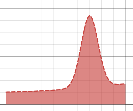
If we choose our sampling points uniformly over the range, only some will be in region where the function is the highest. In other words, there is a reasonable probability that \(f(X)\) is very different to its typical value – so \(\var f(X)\) is large.

To remedy this, let’s remove the assumption that \(X\) is uniformly-distributed. We’ll only assume that its range is \([a, b]\); i.e. its pdf satisfies \(p(x) \neq 0 \Leftrightarrow x \in [a,b]\). We then have

\[\int_a^b f(x)\, dx = \int_a^b \frac{f(x)}{p(x)}\, p(x)\, dx = \E \left[ \frac{f(X)}{p(X)} \right].\]

Now our estimator is

\[\Ih = \frac{b-a}{n} \sum_{i=1}^n \frac{f(X_i)}{p(X_i)}\]

where \(X_1, \dots, X_n\) are distributed like \(X\). Its variance is

\[\var \Ih = \frac{(b-a)^2}{n} \var \left( \frac{f(X)}{p(X)} \right) .\]

This value is low when \(f(x)/p(x)\) does not change much with \(x\). (It is zero in the case the ratio of functions is constant.) Thus, choosing a pdf for \(X\) which has high density where \(f\) is large will result in a smaller estimator variance than the uniform case. It will also result in a faster convergence as the number of samples is increased.

As a final note: Monte Carlo integration is widely applied across mathematics and physics. But interestingly, it is the mathematics behind path tracing in computer graphics; path tracing can be thought of as applying this technique to the rendering equation. Here, importance sampling has the effect of decreasing render time without altering the image!